Shannon Entropy

Welcome! In this post, we’ll explore the concept of Shannon Entropy, a fundamental measure of information in probability theory and information science.

If you are not familiar with probability distributions, you may have a quick review on this probability distribution - quick review.

Definition

Shannon entropy, introduced by Claude Shannon, quantifies the uncertainty or randomness in a data source. It is a fundamental concept in information theory and measures the average amount of information contained in a random variable.

Formula for Shannon Entropy

For a discrete random variable X with n possible outcomes \( \{x_1, x_2, \dots, x_n\} \), each having a probability \( P(x_i) \), the Shannon entropy \( H(X) \) is defined as:

\[ H(X) = -\sum_{i=1}^n P(x_i) \log_b P(x_i) \]

• \( P(x_i) \): Probability of the outcome \( x_i \).
• \( \log_b \): Logarithm with base \( b \) (usually base 2, giving entropy in bits).
• Negative sign ensures that entropy is non-negative since \( P(x_i) \) is between 0 and 1.

Key Intuitions

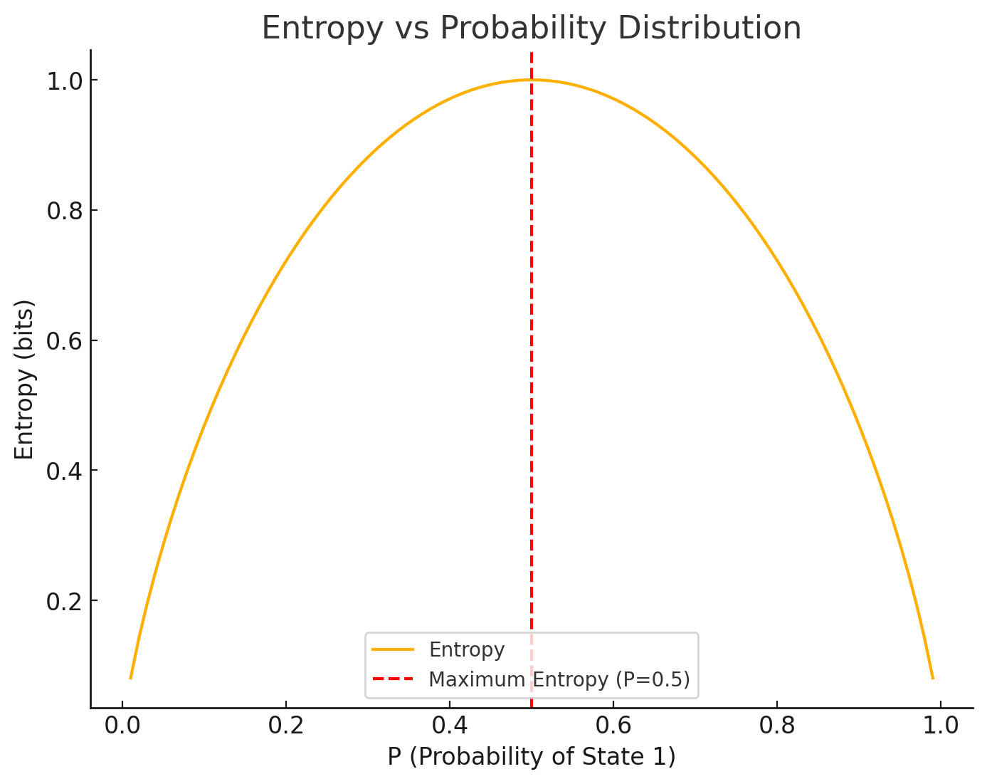
1. Higher Entropy → More Uncertainty

If all outcomes are equally likely, entropy is maximized because we gain the most information by observing the outcome.

2. Lower Entropy → Less Uncertainty

If one outcome is highly likely, entropy is lower because the result is more predictable, so less information is gained.

3. Zero Entropy

When the outcome is completely certain (\( P(x_i) = 1 \) for one outcome and 0 for all others), entropy is zero because there is no uncertainty.

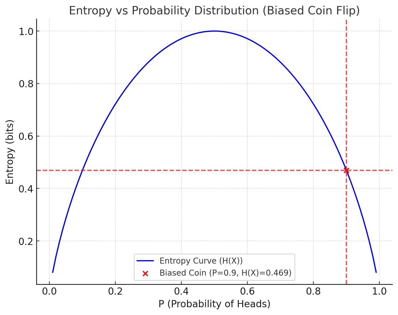
The graph below shows how the entropy varies for one probability state as mentioned above.

Why Logarithms?

a) Logarithms Measure Information Content

The information content \( I(x_i) \) of an outcome \( x_i \) is inversely related to its probability \( P(x_i) \):

\[ I(x_i) = -\log_b P(x_i) \]

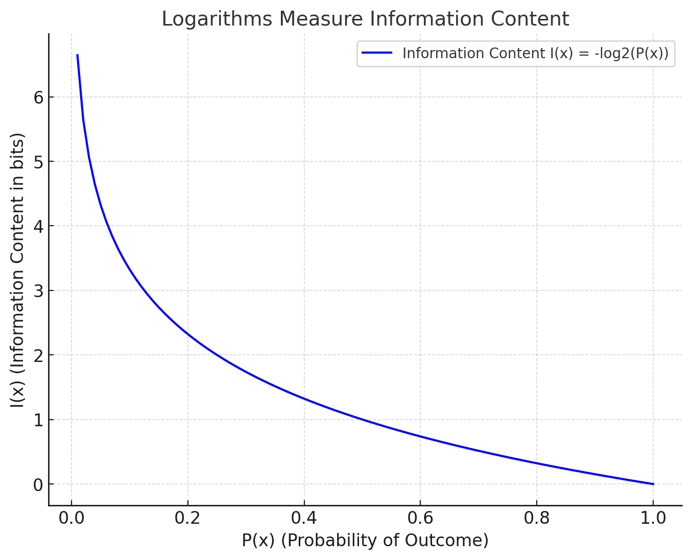
The less likely an event, the more surprising and informative it is.

b) Logarithms Are Additive

The property \( \log_b(xy) = \log_b(x) + \log_b(y) \) makes logarithms suitable for combining uncertainties of independent events.

c) Logarithmic Growth Matches Diminishing Returns

The logarithmic scale reflects diminishing returns in information gain: observing a rare event adds much more information than observing a common one.

Why the Negative Sign?

Probabilities \( P(x_i) \) are between 0 and 1, so \( \log_b(P(x_i)) \) is negative. The negative sign ensures entropy is positive.

Examples

1. Fair Coin Flip

\[ H(X) = - (0.5 \log_2 0.5 + 0.5 \log_2 0.5) = 1 \text{ bit} \]

2. Biased Coin Flip (90% Heads, 10% Tails)

\[ H(X) = - (0.9 \log_2 0.9 + 0.1 \log_2 0.1) \approx 0.469 \text{ bits} \]

3. Uniform Distribution Over 4 Outcomes

If \( P(x_i) = 0.25 \):

\[ H(X) = - (4 \cdot 0.25 \log_2 0.25) = 2 \text{ bits} \]

Explanation of Entropy Differences

1. Fair Coin Flip (\(H(X) = 1 \text{ bit}\))

In a fair coin flip, there is equal probability (\(P(\text{Heads}) = 0.5\)) of landing heads or tails.

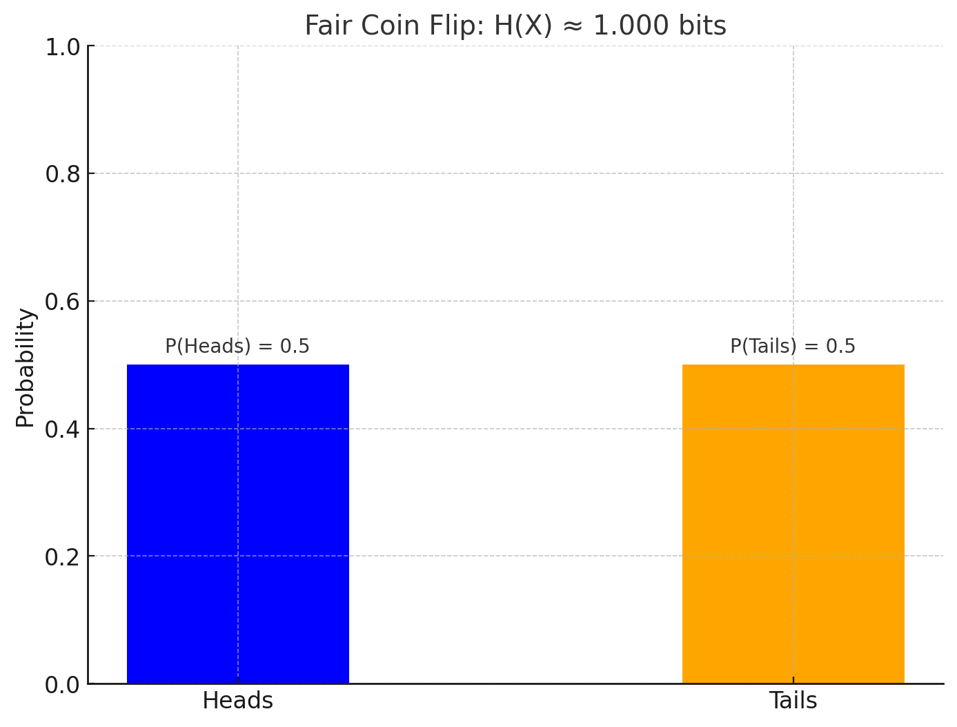
Since both outcomes are equally likely, there is maximum uncertainty; we can't predict the outcome better than pure chance.

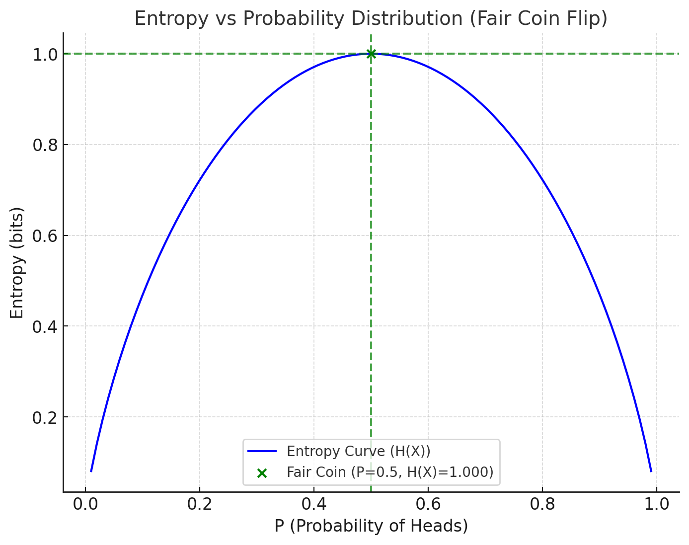
Entropy is highest because there is no bias or preference in the distribution. Each flip carries 1 bit of information.

2. Biased Coin Flip (\(H(X) \approx 0.469 \text{ bits}\))

In this case, one outcome (Heads) is much more likely (\(P(\text{Heads}) = 0.9\)) than the other (\(P(\text{Tails}) = 0.1\)).

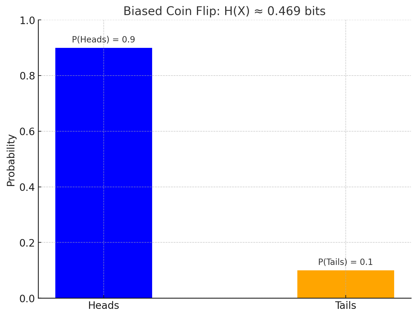
The bias reduces uncertainty because the outcome is more predictable. We can reasonably guess "Heads" most of the time with confidence.

Entropy is lower compared to the fair coin flip because the distribution is uneven, making the system less random.

3. Uniform Distribution Over 4 Outcomes (\(H(X) = 2 \text{ bits}\))

Here, there are four outcomes, each with an equal probability (\(P(x_i) = 0.25\)).

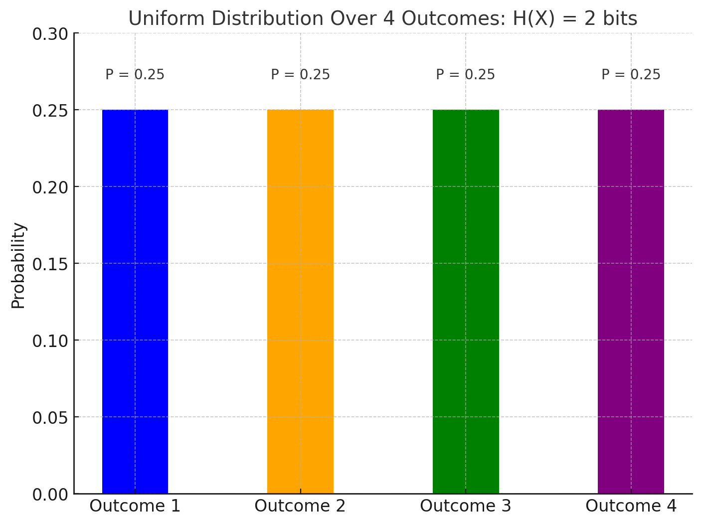
The uncertainty is higher than in the coin flip examples because there are more possible outcomes. Predicting any one outcome is more difficult since each is equally likely.

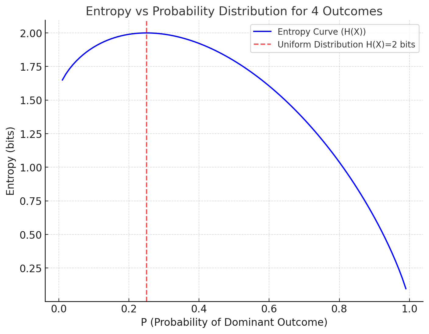
Entropy is maximized for this distribution (given 4 outcomes), as it represents the most random scenario for a uniform probability over four options.

Key Takeaways

• Entropy increases with the number of possible outcomes and is maximized for uniform distributions.
• Entropy decreases when the distribution becomes skewed or biased because predictability increases and randomness decreases.

Why This Formula Works

• Non-Negativity: \( H(X) \geq 0 \), with equality when \( P(x_i) = 1 \) for some \( i \).
• Maximal Entropy for Uniform Distributions: Entropy is maximized when all outcomes are equally likely.
• Additivity: For independent events, \( H(X, Y) = H(X) + H(Y) \).
• Continuity: Small changes in probabilities result in small changes in entropy.

Conclusion

The Shannon entropy formula elegantly captures our intuitive understanding of uncertainty and information. It is fundamental to data compression, cryptography, machine learning, and more.