Probability Distribution - Quick Review

In this post, I’ll cover the fundamental concepts that form the foundation for understanding many topics in other posts on this blog.

Probability and Random Variables

A random variable \( X \) is a variable that can assume a set of possible states or outcomes. Each of these states has an associated probability, which quantifies the likelihood of the random variable taking on that state.

For example, consider a random variable \( X \) that represents the result of flipping a biased coin, which can take two states:

• HEADS
• TAILS

If the probability of observing the outcome HEADS is 70% $$ P(X = \text{HEADS}) = 0.7, $$ then the probability of observing the outcome TAILS is 30%.

\[ P(X = \text{TAILS}) = 1 - 0.7 = 0.3 \]

Which is the rule that all probabilities must sum to 1 (100%). In other words, the probabilities of all possible states must satisfy the following condition:

$$ \sum_{i} P(X = x_i) = 1 $$

This brings us to the concept of a probability distribution, which describes how the total probability of 1 is distributed among the possible states of a random variable.

Probability Distribution

A probability distribution is a function that maps outcomes to their corresponding probabilities. It describes how uncertainty is distributed among individual states in a system and characterizes the system as a whole.

Key Points:

• Total Probability: The total probability of all outcomes must equal 1. Therefore, the probability of one state cannot be changed independently of the others.
• System Characterization: The probability distribution provides a complete description of the system, defining the uncertainty and likelihood of different states.

Examples of Probability Distributions:

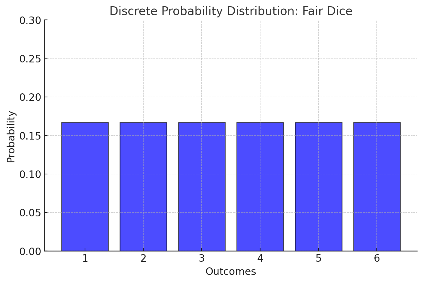
1. Fair Dice (Discrete Random Variable):
   • A discrete random variable consists of distinct states, such as the outcomes of rolling a fair die: {1, 2, 3, 4, 5, 6}.
   • The probabilities of all states must sum to 1:
     \( P(1) + P(2) + P(3) + P(4) + P(5) + P(6) = 1 \)
   • Below is a bar chart representation of the discrete probability distribution:
   
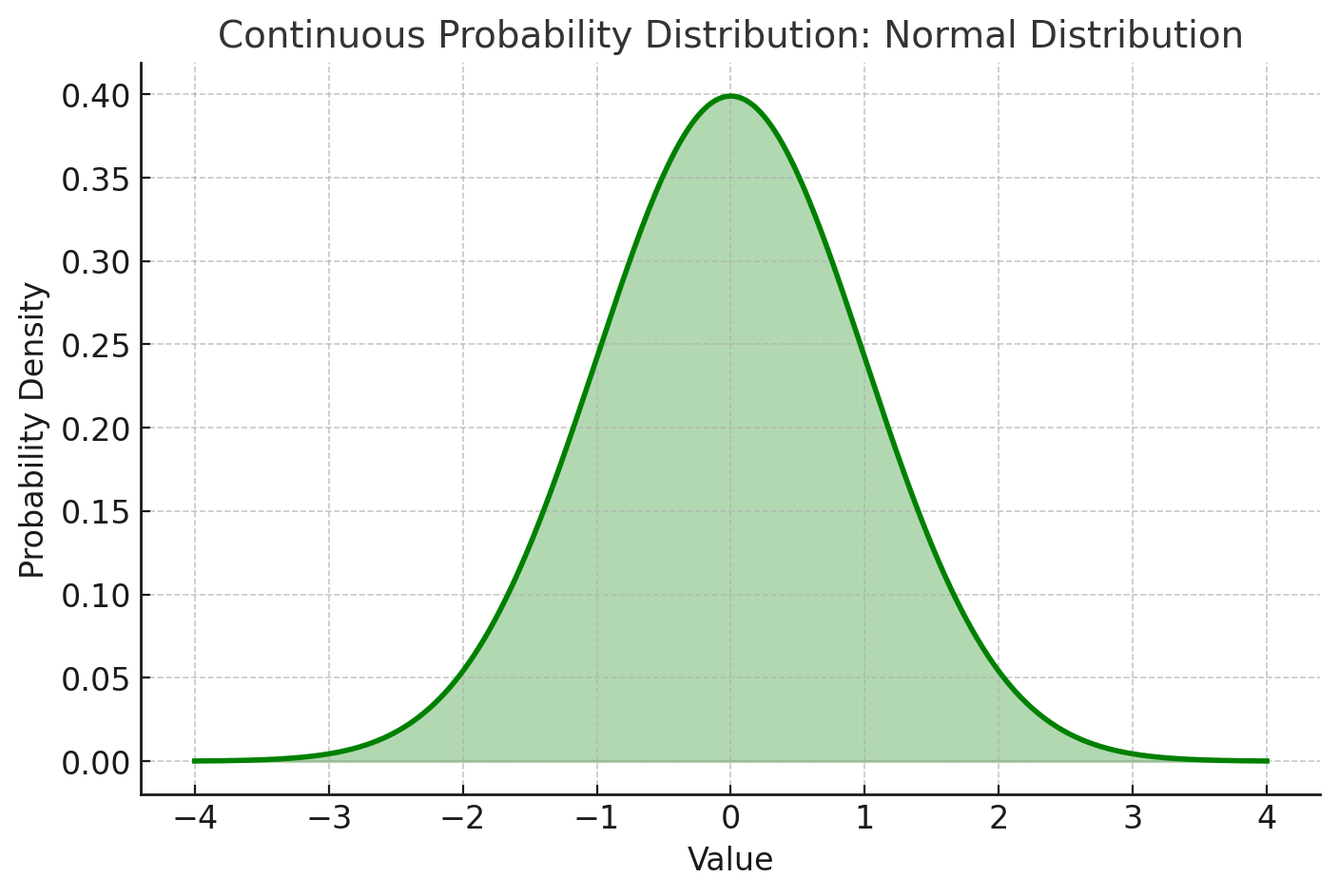
2. Height of Adults (Continuous Random Variable):
   • A continuous random variable represents measurements that can take on any value within a range, such as the height of adults.
   • The total probability is represented by the area under the curve of the probability density function (PDF), which must equal 1: $$ \int_{-\infty}^{\infty} f(x) \, dx = 1 $$
   • Below is a graph representation of the continuous probability distribution (normal distribution):